R-GCN
Modeling Relational Data with Graph Convolutional Networks
2018
首个在KG上应用GNN的模型R-GCN
1 Introduction
一个物品很多的信息隐藏在它的邻居内。R-GCN设计了一个encoder model,可以和其它的tensor factoraction model结合作为decoder。
R-GCN使用了DisMult作为decoder。
在FB15k-237,FB15k,WN18上面都进行了实验。
2 Neural Relational Modeling
2.1 Relational Graph Convolutional Networks
一般的GCN的形式可以定义为 \[ h_i^{l+1}=\sigma(\sum_{m \in M_i}g_m(h_i^{l}, h_j^{l})) \] \(g_m\)可以是neural network,也可以是简单的线性转换,\(g_m(h_i, h_j)=Wh_j\)
基于以上的原理,设计了如下的传播层: \[ h_i^{l+1}=\sigma(\sum_{r\in R}\sum_{j\in N_i^r} \frac{1}{c_{i,r}} W_r^{l}h_j^{l} + W_o^l h_i^l) \] 公式中的\(c_{i,r}\)可以为\(|N_i^r|\),某个关系r的邻居的数量。
以下公式非论文原本内容 \[ h_i^{l+1}=\sigma(\sum_{r\in R}\sum_{j\in N_i^r} \frac{1}{\sqrt{c_{i}} \sqrt{c_{j}}} W_r^{l}h_j^{l}) \]
\[ h_i^{l+1}=\sigma(\sum_{r\in R}\sum_{j\in N_i^r} \frac{1}{\sqrt{c_{i}} \sqrt{c_{j}}} W_r^{l} [h_j^{l},e_r^{l}]) \]
2.2 Regularization
这样设计导致了不同层的不同关系都有不同的weight matrix,在large scale knowledge graph下会导致快速增加的参数数量,导致过拟合。
为此,R-GCN使用了两种正则方式,都是针对\(W_r^l\)进行改进。
basis- and block-diagonal decomposition
1、basis decomposition: \[ W_r^l=\sum_b^B a_{r,b}^l V_b^l \] \[ V_b^l \in R^{d^{(l+1)}\times (d^l)} \]
这种情况下\(W_r^l\)成为线性组合同一层的不同关系,能够共享\(V_b^l\),区别在于\(a_{r,b}^l\)。
The basis function decomposition can be seen as a form of effective weight sharing between different relation types
这种方式可以看做是有\(B\)个矩阵\(V\),然后与邻居实体embedding相乘,得到\(B\)个message embedding,然后对于不同的关系使用权重\(a_{1,b}^l,\dots,a_{B,b}^l\)去聚合。
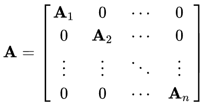
2、block-diagonal decomposition \[ W_r^l=\oplus_b^B Q_{b,r}^l \]
\[ W_r = diag(Q_{1r}^{l},\cdots,Q_{Br}^{l})\ with\ Q_{br}^{l} \in \mathbb{R}^{(d^{l+1}/B)\times (d^{l}/B)} \]
其中符号\(\oplus\)是矩阵加法中的Direct Sum,不是普通的相加,而是下面的形式,
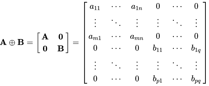
这里说明下block-diagonal matrix,根据维基百科的解释
A block diagonal matrix is a block matrix that is a square matrix such that the main-diagonal blocks are square matrices and all off-diagonal blocks are zero matrices.
对于这种正则化方式的理解
The block decomposition can be seen as a sparsity constraint on the weight matrices for each relation type.
它与bias decomposition的区别是它没有设置共享参数的结构,而是直接使用更加系数的\(W_r\)去拟合。
3 Entity Classification
对于实体分类,就是将entity 分类为K个class当中,那么在R-GNN的基础上,直接在最后一层的输出增加softmax就可以,训练时的loss为 \[ L=-\sum_{i\in Y}\sum_{k=1}^{K}t_{ik}lnh_{ik}^L \] \(Y\)是所有有label的entity集合。
4 Link Prediction
要进行Link Prediction,在R-GCN的基础上需要设计一个score function。
论文直接使用了DistMult作为decoder, \[ f(s,r,o)=e_s^TRe_o \] 训练的loss为 \[ L=-\frac{1}{(1+w)|\varepsilon|}\sum_{(s,r,o,y)\in \Gamma}{ylog(f(s,r,o)) + (1-y)log(1-f(s,r,o)) } \] 前面的系数为归一系数,\(w\)为对于每一个postivite sample取\(w\)个negative samples,\(|\varepsilon|\)为所有实体的个数。
5 Empirical Evaluation
5.1 Entity Classification Experiments
数据集
- AIFB
- MUTAG,
- BGS
- AM
超参设计
- 2-layer model with 16 hidden units
- basis function decomposition
- Adam,learning rate of 0.01
Baseline:
RDF2Vec embeddings
WeisfeilerLehman kernels (WL)
hand-designed feature extractors (Feat)
5.2 Link Prediction Experiments
| Dataset | WN18 | FB15K | FB15k-237 |
|---|---|---|---|
| Entities | 40,943 | 14,951 | 14,541 |
| Relations | 18 | 1,345 | 237 |
| Train edges | 141,442 | 483,142 | 272,115 |
| Val. edges | 5,000 | 50,000 | 17,535 |
| Test edges | 5,000 | 59,071 | 20,466 |
FB15k-237是FB15K的reduced版本,去除了所有的inverse relation。
评估指标:
- MRR
- HIT@